
Introduction
As developers of pairs trading execution software for the past 17 years, we found that the term ‘pairs’ is a somewhat nebulous catchall phrase for many different trading strategies. These include risk (or merger) arbitrage, statistical arbitrage, cross border arbitrage, dual share class arbitrage, leveraged ETF arbitrage, inverse ETF arbitrage, multi-legged spinoff arbitrage, various ‘long/short’ strategies and others. Developing tools for all of these strategies has been interesting and fun, with plenty of challenges. We thought it might be interesting to address some of the math behind the execution of the various strategies.
Because these trading strategies evolved as separate disciplines, it is not surprising that most of them have their own way of looking at the strategy along with separate terminology. The distinction is so great, that some of our customers don’t even consider themselves ‘pairs’ traders.
When developing software for similar but different strategies, one must try to understand the commonality of the strategies and design an underlying model that accommodates as much of it as possible. Having a good underlying model as a base makes a huge difference in a whole lot of ways that are critically important to building dynamic software products.
Although there is much more to a pairs trading execution platform than the underlying math, it is an important component and the subject of this multi-part article. None of the math is complex, but some of the scenarios make things a bit complicated. In this first article, we’ll focus on basic pricing for a couple of simple strategies, then address specific strategies more thoroughly in subsequent articles.
A Risk Arbitrage Example
Let’s look at a couple of examples of basic pairs trading strategies and then try to see what they have in common.
Risk arb involves one company acquiring another company, often by exchanging its own shares for those of the target company at a specified ratio with some sort of cash component. (Deals can be lots more complicated, but we will use a simple one for our purposes.) The trader wants to execute the appropriate amount of the two securities at the correct relative prices, so the execution platform will need to know the correct relative prices of the two securities at any given point in time.
Typically a trader would short the acquirer (Company A) and buy the target (Company B) at some discount to the ‘fair value’ represented by the terms of the deal. So, let’s say company A will acquire company B. Company B will receive .44 shares of Company A plus $4.50 in cash. Let’s say the trade wants to make .50. So, the general formula would be:
Target Company price = (Acquirer Company Price * Share Ratio) + (Cash Component – Trader’s Profit).
So in this example, the formula becomes:
Company B Price = (Company A price *.44) + ($4.50 - .50).
Let’s throw these into a spreadsheet and calculate the price we would be willing to pay for Company B for a range of prices for Company A.
Terms:
| Ratio | Cash | Profit Target |
|---|---|---|
| .44 | 4.50 | .50 |
Target price of Company B for range of prices of Company A.
| Company A | Company B |
|---|---|
| 50.00 | 26.00 |
| 50.50 | 26.22 |
| 51.00 | 26.44 |
| 51.50 | 26.66 |
| 52.00 | 26.88 |
| 52.50 | 27.10 |
| 53.00 | 27.32 |
| 53.50 | 27.54 |
| 54.00 | 27.76 |
| 54.50 | 27.98 |
| 55.00 | 28.20 |
| 55.50 | 28.42 |
| 56.00 | 28.64 |
| 56.50 | 28.86 |
| 57.00 | 29.08 |
| 57.50 | 29.30 |
Here’s a chart showing the relationship.
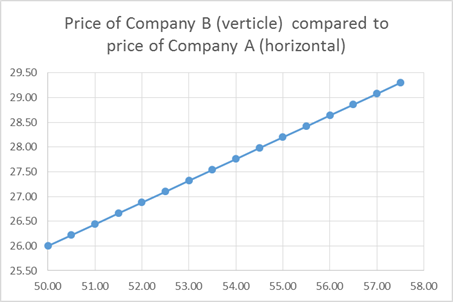
So, we see the relative prices we would like to execute are linear for this risk arbitrage example. Hold that thought for a moment and let’s move on to another pairs strategy, statistical arbitrage.
A Statistical Arbitrage Example
There are lots of different variants of statistical arbitrage strategies, but let’s take a look at a simple one. Let’s say that someone has done some research and found that prices of two companies in the same industry tend to track one another very closely but at times one or the other will drift higher or lower relative to the other one and then drift back to the norm.
Here’s an example of two such stocks. We’ll call them Company A and Company B. The top part of the chart shows their prices (one on each vertical access) and the bottom chart shows the premium or discount to their previous year’s average ratio.
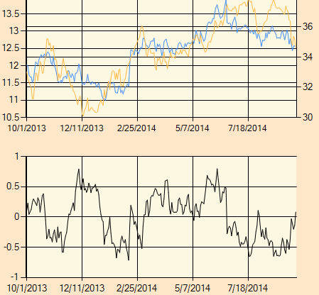
A trading strategy might be to buy the pair when it gets to a .50 discount and sell it when it gets to a .50 premium. Let’s set up the math on this one. Let’s buy when
Company B Price = (Company A Price * Average Ratio) – Target Discount
and sell when
Company B Price = (Company A Price * Average Ratio) + Target Discount
So, if we fill in the numbers, we buy when
Company B = (Company A * .3610) - .50
and sell when
Company B = (Company A * .3610) + .50
Let’s put the data into a table across a range of values for Company A and see where we should execute Company B for any given price to both put on and take off the position.
| Buy | Sell | |
|---|---|---|
| Company A | Company B | Company B |
| 31.00 | 10.69 | 11.69 |
| 31.50 | 10.87 | 11.87 |
| 32.00 | 11.05 | 12.05 |
| 32.50 | 11.23 | 12.23 |
| 33.00 | 11.41 | 12.41 |
| 33.50 | 11.59 | 12.59 |
| 34.00 | 11.77 | 12.77 |
| 34.50 | 11.95 | 12.95 |
| 35.00 | 12.14 | 13.14 |
| 35.50 | 12.32 | 13.32 |
| 36.00 | 12.50 | 13.50 |
| 36.50 | 12.68 | 13.68 |
| 37.00 | 12.86 | 13.86 |
| 37.50 | 13.04 | 14.04 |
| 38.00 | 13.22 | 14.22 |
| 38.50 | 13.40 | 14.40 |
And the corresponding chart.

So, our statistical arbitrage example also has a linear relationship.
Remember 7th Grade Algebra?
We’ve looked at two simple pairs trading strategies and observed a linear relationship in both of them. Let's go back to our 7th grade algebra class. Remember this?
y = mx + b
Now let’s look at our three formulas from earlier. The risk arbitrage one:
Company B Price = (Company A price *.44) + ($4.50 - .50).
And the two for our stat arb example:
Company B = (Company A * .3610) - .50
Company B = (Company A * .3610) + .50
These three equations seem to fit nicely with y = mx + b, and the linear look of the charts seem to confirm. So, if we were to build an model for pairs execution strategies, it looks like a linear equation defining the underlying relationship would be a good place to start. In our next posting, we’ll go into more depth on a couple of statistically arbitrage strategies and introduce the (simple) math on how to manage volume. Subsequent posts will deal with more complex pairs strategies.